Getting started with scRNA-seq

Quick start guide

See vignette("authentication") for instructions on creating your personal API token for accessing data. To begin using pluto, load the package and log in with your personal API token:

library(pluto)
pluto_login("<YOUR API TOKEN>")

Accessing `Seurat` objects from Pluto

Single cell RNA-seq in Pluto creates two Seurat objects: a raw Seurat object, which is created at the beginning of the single cell RNA-seq preprocessing workflow and has not been filtered, normalized, integrated, clustered, etc.; and a final Seurat object, which is the final, processed Seurat object that results from completing and accepting a preprocess workflow. Both Seurat objects are accessible for external scRNA-seq analysis via the pluto package.

Download Seurat object

To download a Seurat object, provide the experiment ID, Seurat type ("raw" or "final") to the pluto_download_seurat_object() function (you can also provide an optional desired destination file path by setting dest_filename):

experiment_id <- "PLX037839"
seurat_type <- "raw"
pluto_download_seurat_object(experiment_id, seurat_type)

Read `Seurat` object

To read a Seurat object directly into your R script, provide the experiment ID and Seurat type ("raw" or "final") to the pluto_read_seurat_object() function:

experiment_id <- "PLX037839"
seurat_type <- "raw"
so <- pluto_read_seurat_object(experiment_id, seurat_type)

It is important to note that the pluto_read_seurat_object() function returns different objects depending on the Seurat type specified. If the Seurat type is specified as "raw", a Seurat object will be returned. If the Seurat type is specified as "final", a list is returned containing the final Seurat object, obj, with custom cluster annotations added to the Seurat meta.data and custom color palettes corresponding to the cluster annotation sets in-app, colors.

experiment_id <- "PLX037839"
seurat_type <- "final"
final_obj <- pluto_read_seurat_object(experiment_id, seurat_type)

# To access the Seurat object
so <- final_obj$obj

# To access the custom color palettes
custom_palettes <- final_obj$colors

The `Seurat` object

The Seurat object, developed by the Satija lab, is a representation of single-cell expression data for R. The object serves as a container that contains both data (like the count matrix) and analysis (like PCA, or clustering results) for a single cell dataset. At the top level, the Seurat object serves as a collection of Assay and DimReduc objects, representing expression data and dimensionality reductions of the expression data, respectively. Seurat objects also store additional metadata, both at the cell and feature level. Click here for more information.

To access your Seurat object assay(s):

so@assays

To access your Seurat object reductions:

so@reductions

To access your Seurat object meta.data:

so@meta.data

# Or, to just display the first n rows of meta.data:
head(so@meta.data, n = 10)

The column names in your meta.data will correspond to the variables and latent variables you see in the Pluto app. You will also see additional columns that were added during the preprocess workflow, mostly related to QC. If you are reading in a final Seurat object, you will see columns that correspond to your cluster annotation sets.

To get a list of available meta.data columns in your Seurat object:

colnames(so@meta.data)

Visualization using the `Seurat` package

Once a Seurat object has been downloaded from Pluto, we can use a variety of base plotting functions from the Seurat package. We can further modify and customize these plots using ggplot2.

library(Seurat)
library(ggplot2)
library(ggridges)

Dimensional reduction plot

Using the Seurat DimPlot() function, make a scatter plot in UMAP space grouping cells by custom annotation set “Default cluster - res. 0.1” (here, we can use one of our custom color palettes that we defined in the Pluto app):

DimPlot(so, # the Seurat object
     reduction = "umap", # could also be "tsne" or "pca"
     group.by = "default_clusters_res_0_1", # custom annotation set
     cols = custom_palettes$default_clusters_res_0_1, # custom color palette
     pt.size = 0.1
) + # point size for plotting
     labs(
          title = "Default clusters - res. 0.1", # update plot title
          x = "UMAP 1", # update x-axis label
          y = "UMAP 2"
     ) # update y-axis label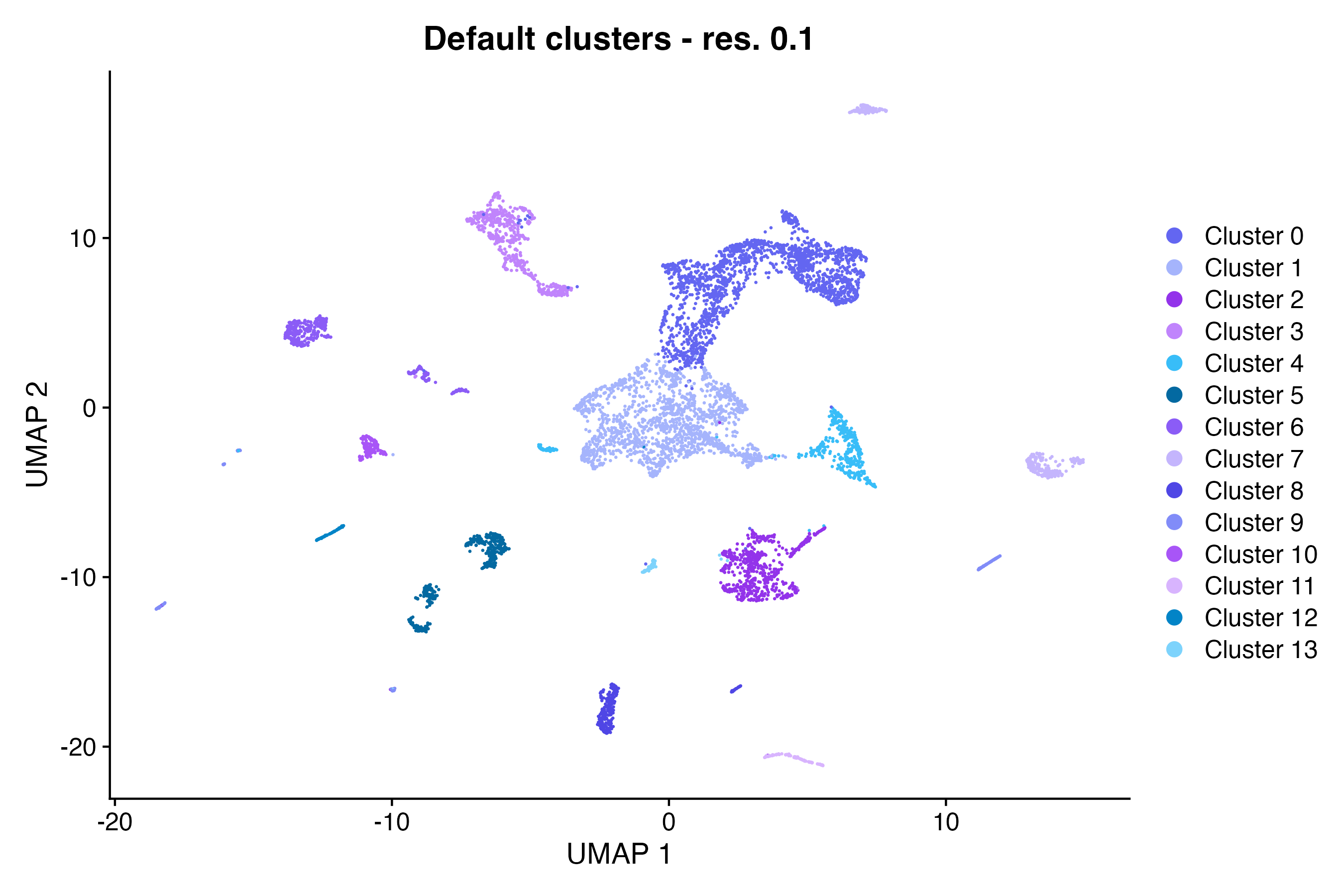

Using the Seurat DimPlot() function, make a scatter plot in UMAP space grouping cells by timepoint:

# Create a custom color palette to group cells by timepoint
timepoint_cols <- c("#14b8a6", "#fcd34d", "#ef4444")
names(timepoint_cols) <- c("24hpf", "36hpf", "48hpf")

DimPlot(so, # the Seurat object
     reduction = "umap", # could also be "tsne" or "pca"
     group.by = "timepoint", # available column in our meta.data, from our Pluto sample data
     cols = timepoint_cols,
     pt.size = 0.1
) + # point size for plotting
     labs(
          title = "Timepoint", # update plot title
          x = "UMAP 1", # update x-axis label
          y = "UMAP 2"
     ) # update y-axis label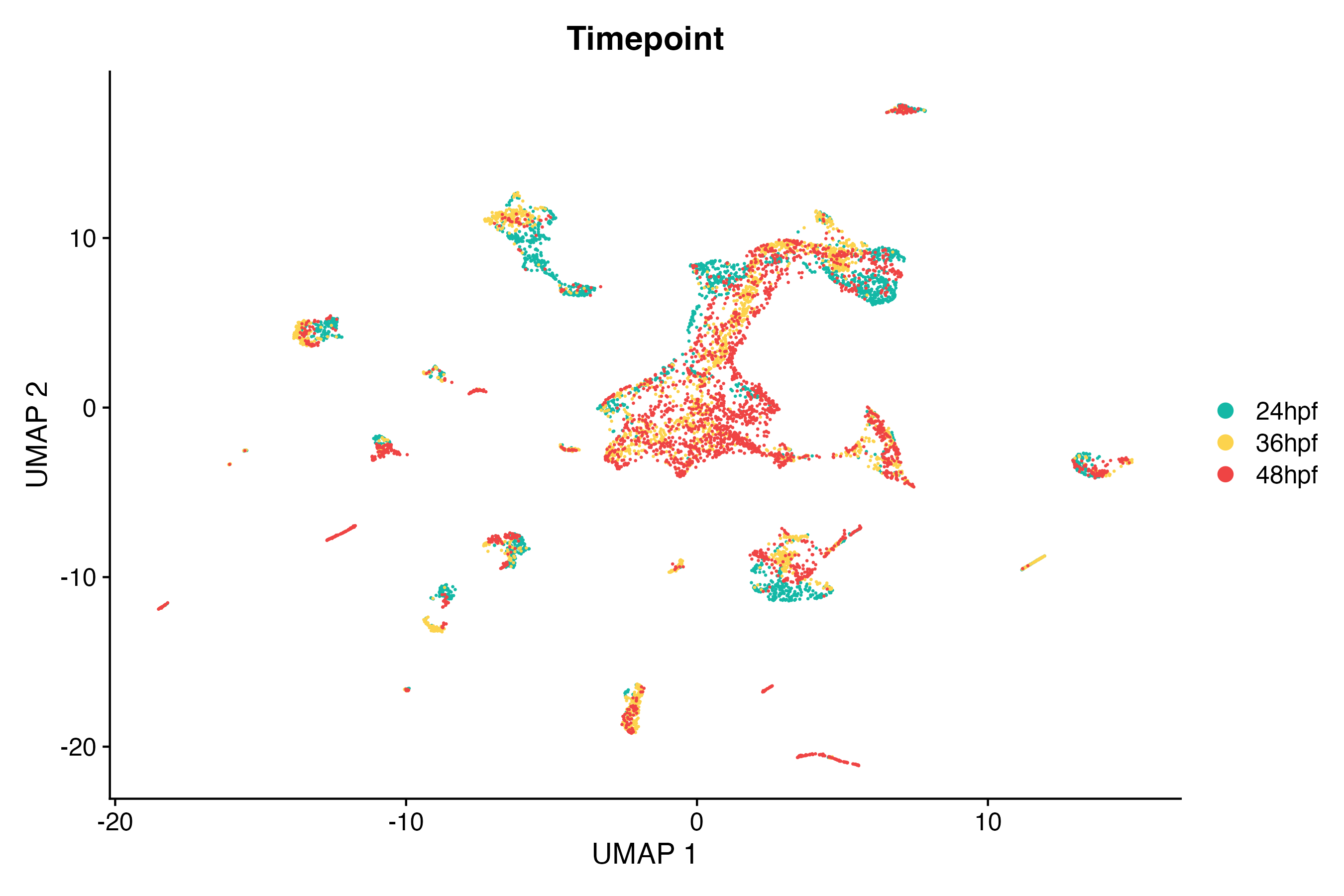

Using the Seurat DimPlot() function, make a scatter plot in UMAP space grouping cells by custom annotation set “Default cluster - res. 0.1” and splitting cells by timepoint:

DimPlot(so, # the Seurat object
     reduction = "umap", # could also be "tsne" or "pca"
     group.by = "default_clusters_res_0_1", # custom annotation set
     cols = custom_palettes$default_clusters_res_0_1, # custom color palette
     split.by = "timepoint", # custom annotation set
     pt.size = 0.1
) + # point size for plotting
     labs(
          title = "Default clusters - res. 0.1", # update plot title
          x = "UMAP 1", # update x-axis label
          y = "UMAP 2"
     ) # update y-axis label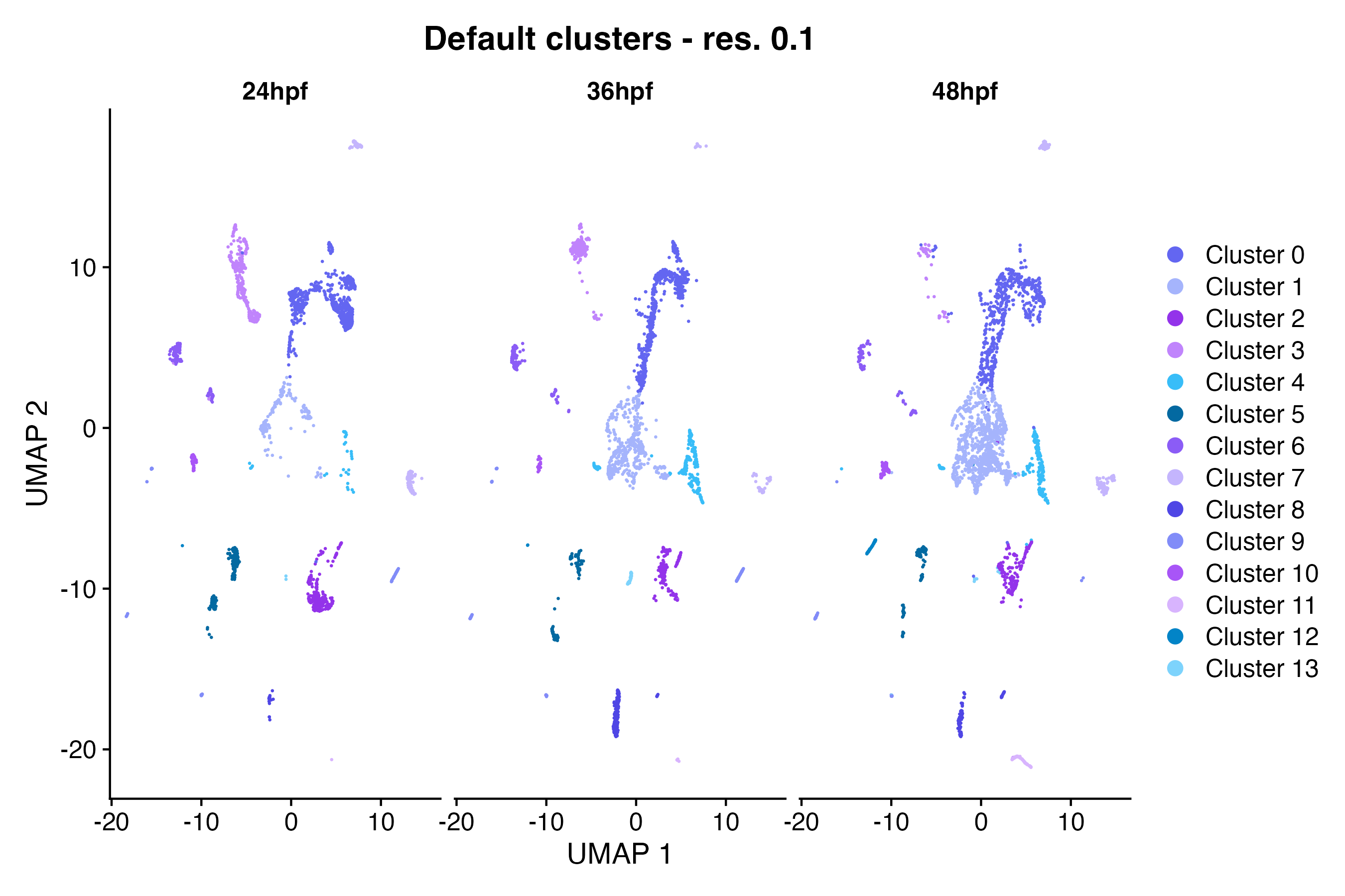

Marker feature expression

Violin plot

Using the Seurat VlnPlot() function, make a violin plot grouping cells by custom annotation set “Default cluster - res. 0.1”:

VlnPlot(so, # the Seurat object
     features = c("olig2"), # feature(s) of interest
     group.by = "default_clusters_res_0_1", # custom annotation set
     cols = custom_palettes$default_clusters_res_0_1
) + # custom color palette
     labs(
          title = "Expression of olig2", # update plot title
          x = "Default clusters - res. 0.1"
     ) # update x-axis label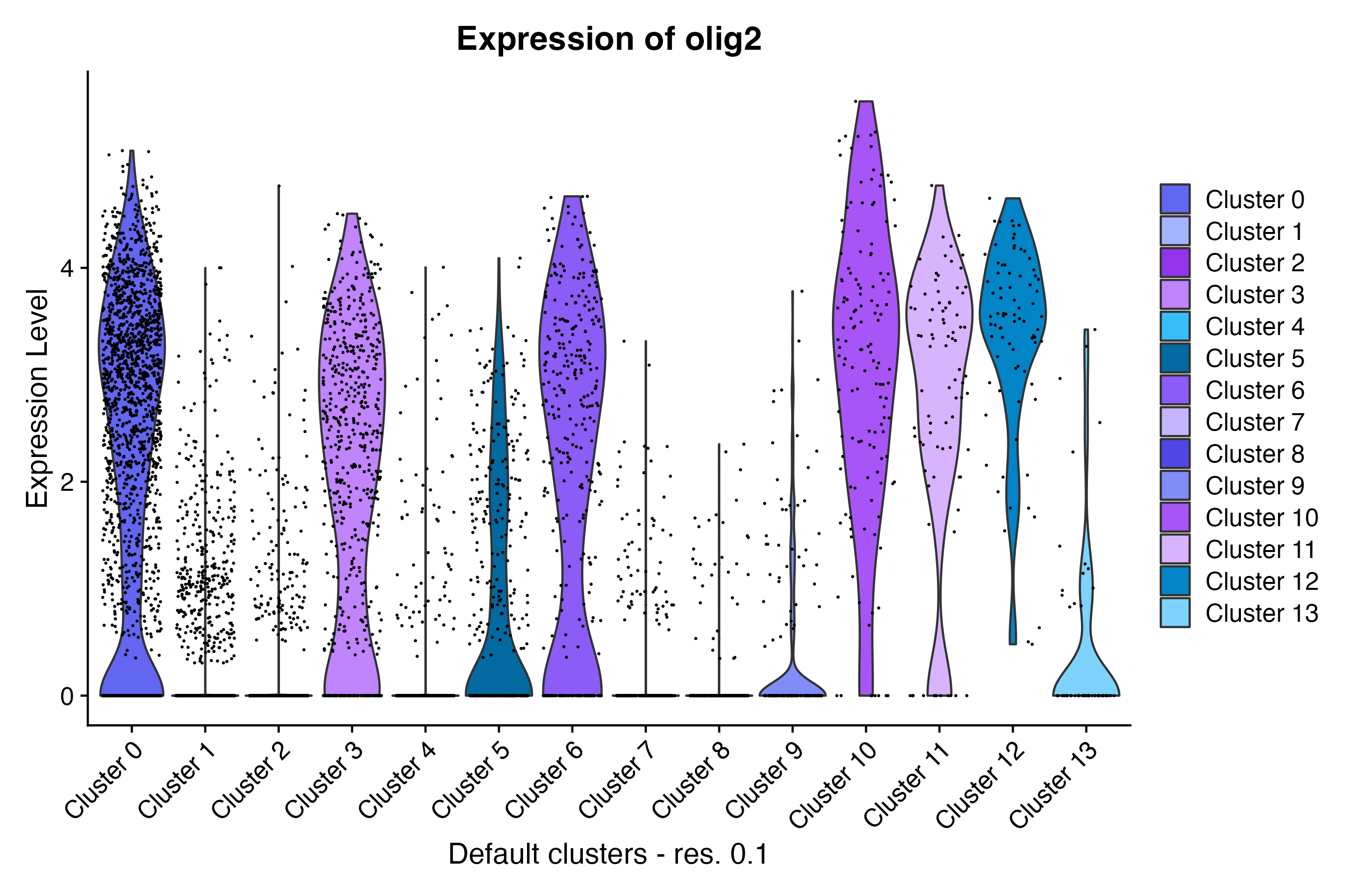

Ridge plot

Using the Seurat RidgePlot() function, make a ridge plot grouping cells by custom annotation set “Default cluster - res. 0.1”:

RidgePlot(so, # the Seurat object
     features = c("olig2"), # feature(s) of interest
     group.by = "default_clusters_res_0_1", # custom annotation set
     cols = custom_palettes$default_clusters_res_0_1
) + # custom color palette
     labs(
          title = "Expression of olig2", # update plot title
          y = "Default clusters - res. 0.1"
     ) + # update x-axis label
     theme_ridges(center = TRUE) # center the x and y axis labels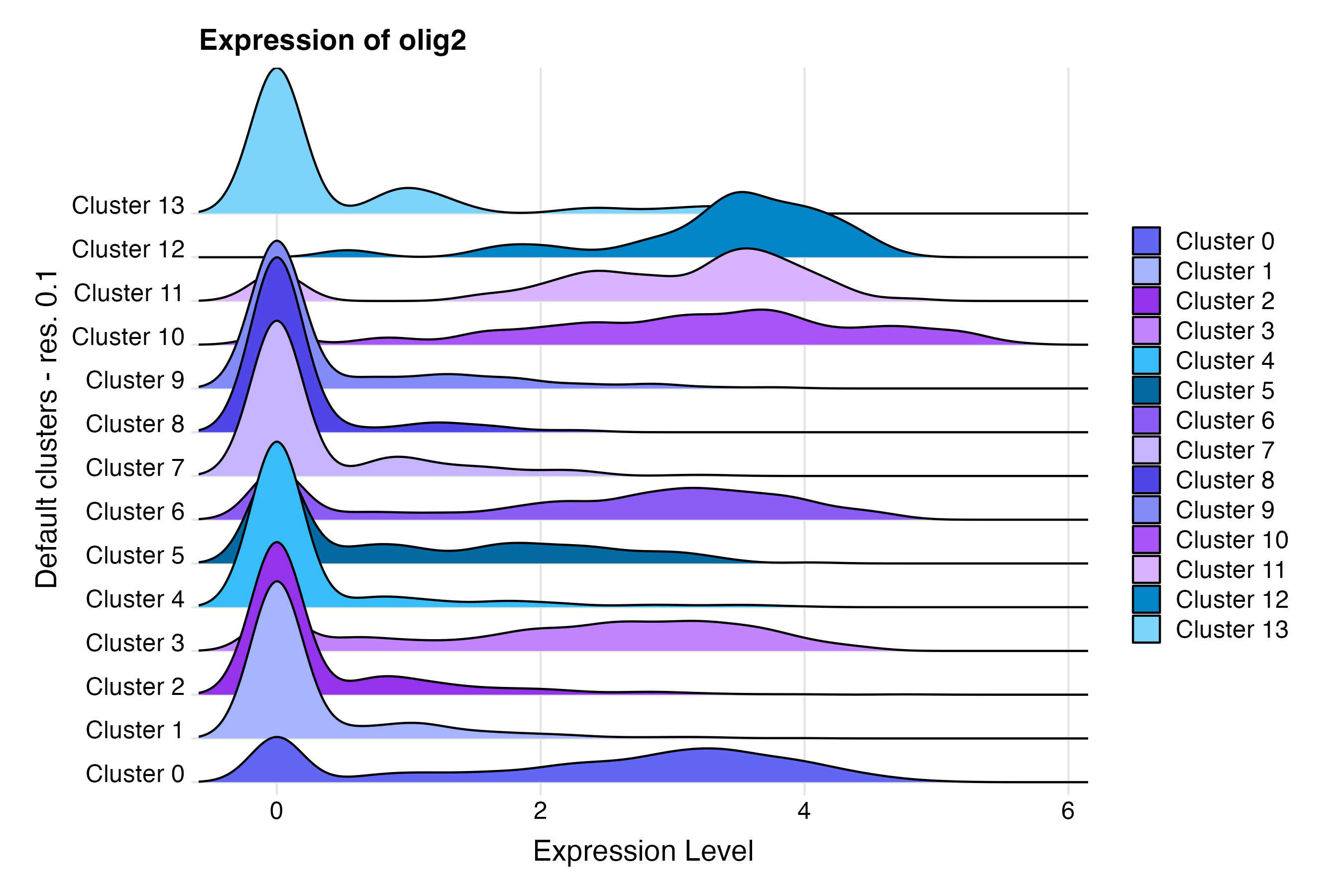

Feature plot

Using the Seurat FeaturePlot() function, make a scatter plot in UMAP space colored by feature expression:

FeaturePlot(so, # the Seurat object
     features = c("olig2"), # feature(s) of interest
     reduction = "umap", # could also be "tsne" or "pca"
     pt.size = 0.1
) + # point size for plotting
     labs(
          title = "Expression of olig2", # update plot title
          x = "UMAP 1", # update x-axis label
          y = "UMAP 2"
     ) # update y-axis label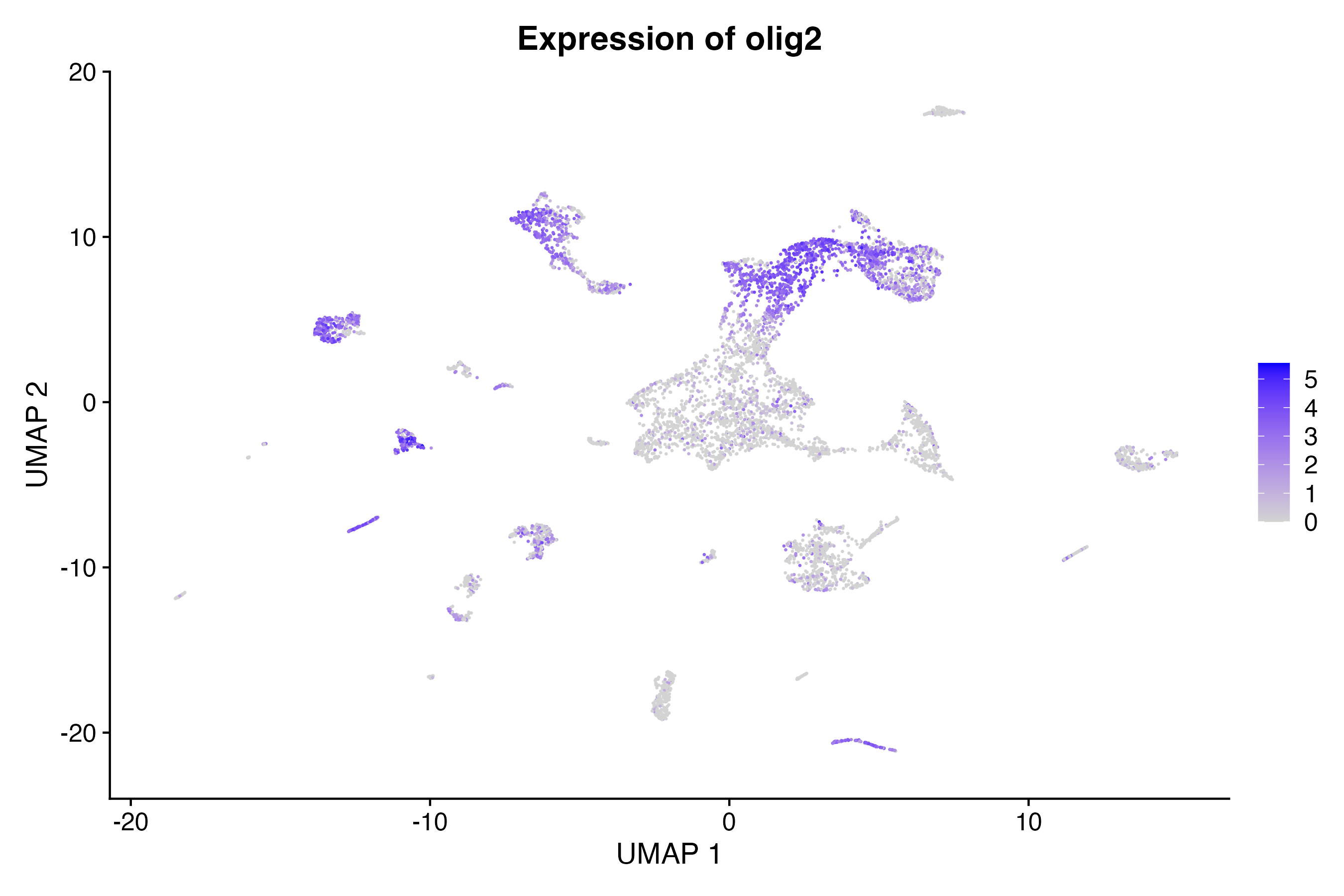

Dot plot

Using the Seurat DotPlot() function, make a dot plot colored by feature expression:

DotPlot(so, # the Seurat object
     features = c("olig2", "sox19a", "gfap", "dlb", "nkx2.2a"), # feature(s) of interest
     group.by = "default_clusters_res_0_1"
) + # custom annotation set
     labs(
          title = "Key marker genes", # update plot title
          x = "Genes", # update x-axis label
          y = "Default clusters - res. 0.1"
     ) # update y-axis label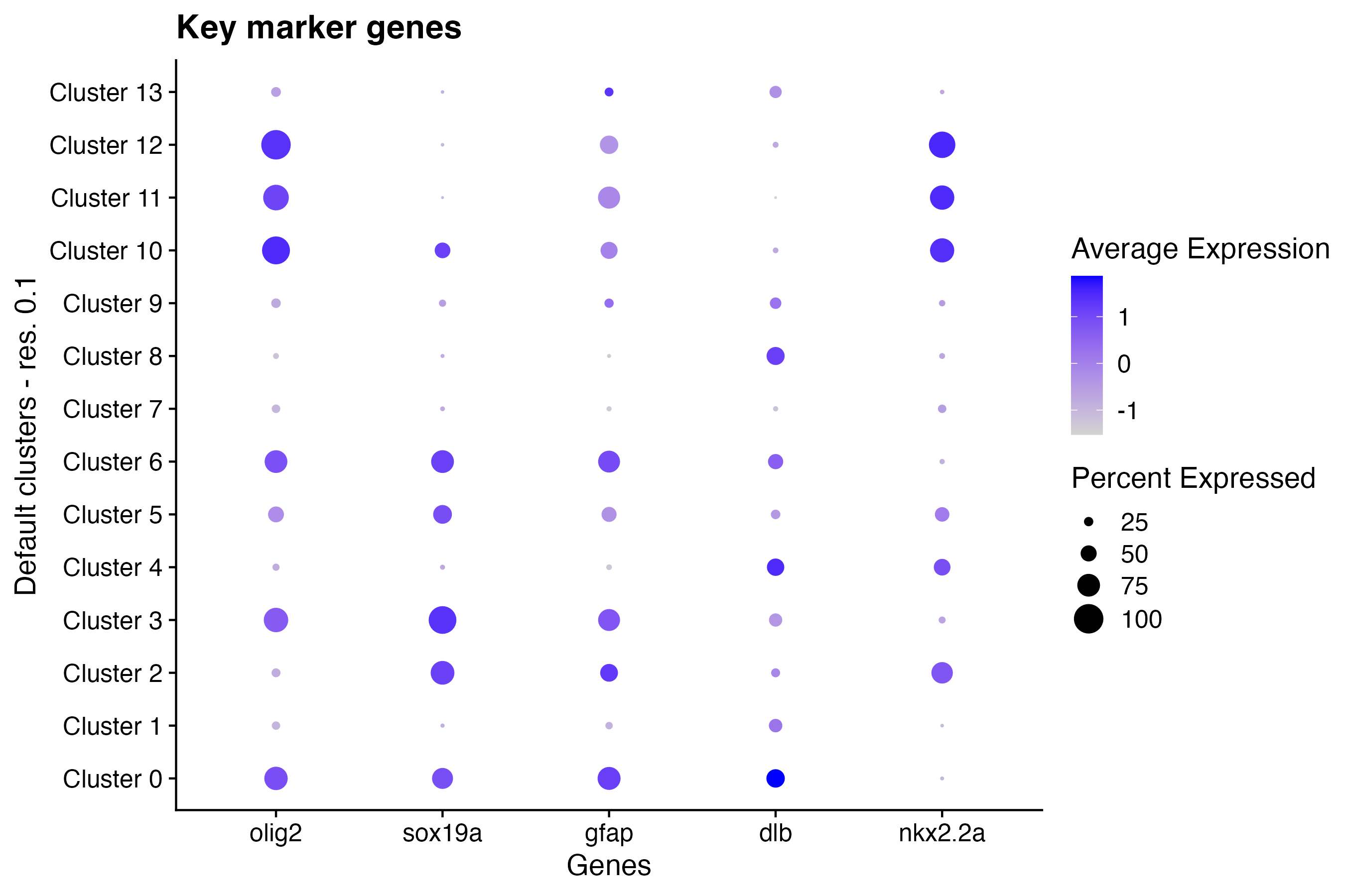

For more visualization tutorials using the Seurat package, check out the Seurat visualization vignette here.